
 |
| Characterization and Modeling of Non-linear Behavior of Plastics |
|
||
Hubert Lobo DatapointLabs, Ithaca, NY and Juan A Hurtado ABAQUS, Inc., Providence, RI |
|||
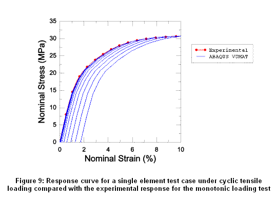
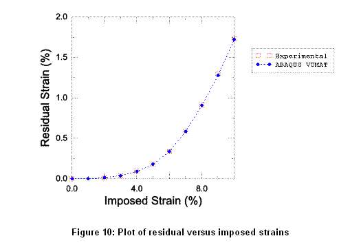
Abstract A considerable amount of CAE today is devoted to the simulation of non-metallic materials, many of which exhibit non-linear behavior. However, most material models to date are still based on metals theory. This places severe restrictions on the proper description of their behavior in CAE. In this paper, we describe non-linear elastic behavior and its interrelationship with plastic behavior in plastics. Special attention is given to the differentiation between visco-elastic (recoverable) strain and plastic (non-recoverable) strain. The goal of this work is to have a material model for plastics that can describe both loading and unloading behavior accurately and provide an accurate measure of damage accumulation during complex loading operations. Keyword: non-linear elasticity, plasticity, plastic point, yield point, true yield point, damage accumulation, residual strain. Introduction When designing plastic parts, it is often important to know at what strains and stresses the material fails. Plastics are dramatically different from metals in their stress-strain behavior. Unlike metals, they undergo significant strain prior to yielding, often as high as 5 to 7%. A significant portion of this strain can be plastic in nature. Plastic deformations cause irreversible damage in the part and it is dangerous to assume that the plastic is stable up to its yield point. This places considerable difficulty for the analyst because first, it is not trivial to differentiate between recoverable strain and plastic strain. Secondly, it is important to know at what strain and stress level these deformations start to be significant. Thirdly, simulation of damage accumulation and recovery after loading are not feasible unless the relationship between recoverable strain and plastic strain is known. A common mechanical test for plastics is the tensile test. A specimen is stretched at a constant speed, and the forces are recorded. A stress-strain curve can then be derived. Often the yield point, the maximum of the stress strain curve, is assumed to be synonymous with the onset of plastic deformation. This concept is erroneous, as it has been shown that plastic flow starts before this point. This maximum on the curve actually corresponds to the point where the specimen becomes unstable and a neck forms. The stress-strain curve can then be decomposed in the following regions shown in Figure 1 and described by Courtney (1991): -The first region corresponds to viscoelastic (recoverable) deformations. -The second region starts at what we will now call the plastic point of the material. Plastic deformations become significant, through crazes formations and/or homogeneous flow (shear bands). -The third region corresponds to the formation of a neck in the specimen. The deformation is dominated by a massive homogeneous flow in the drawing regions. 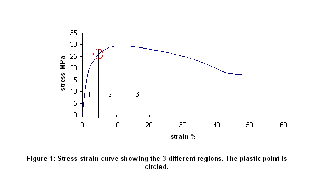 Two other factors need to be mentioned which further complicate the problem. Plastics exhibit non-linear elasticity. As seen in Figure 1, there is often no linear portion to the initial stress-strain curve. Instead, the tangent modulus is seen to steadily decrease with increasing strain all the way to the yield point. At the plastic point, the plastic begins to take on irrecoverable plastic strain. Such behavior plays havoc with the classical elastic-plastic material model because it is often grossly incorrect to use a secant modulus to describe the elastic stress-strain relationship below the plastic point. While such a model has some applicability for the simulation of large deformations, it will show the material to be soft at low strains. See Figure 2. 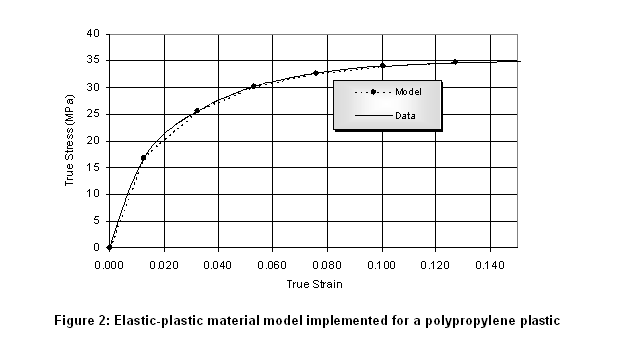 Lastly, the issue of visco-elasticity cannot be ignored. Even in the so-called elastic region, the recovery of a plastic subject to deformation is not instantaneous. Rather, the plastic returns to it's original state after a period of time that is dependent on its visco-elastic characteristics, as described by a stress-relaxation curve. This time dependency is well characterized by visco-elastic experiments and can be modeled well in high end CAE applications via a Prony series. However, visco-elastic theory implemented in most CAE programs is a linear theory and therefore unsuitable for large-strains where the visco-elastic behavior itself becomes non-linear. As permanent irrecoverable plastic strain occurs, the material itself is changed and now has a new characteristic that is entirely different from the original material. Accordingly, linear visco-elastic models will not work beyond the plastic point. In order to shed some light on this problem, we conducted a series of experiments following the work of Quinson (1996). Details are provided in the Experimental Scheme section. The resulting test data yielded the residual plastic strain for a series of imposed strains. To describe the mechanical behavior of this material we propose a constitutive model based on multiplicative finite-strain elastoplasticity. The calibration procedures and validation of the model are discussed in the Material Modeling section. Experimental Scheme The general idea of the procedure is to load the specimen, let it relax and measure the residual deformations after a fixed period of time. This procedure has been used previously by Quinson (1996, 1997) with success on PMMA, PS and PC. In their work, several test specimens were deformed up to different strain levels, and then unloaded and measured after a given recovery time of 8-24 hours. The residual strains could then be plotted as a function of the initially applied strains. When the initial deformation had exceeded the plastic limit of the material, a dramatic increase of residual strain was observed. It had also been shown by Quinson (1997) that this limit was independent on the time allowed for the material to recover. In order to improve the feasibility of the test procedure we exploited this finding to reduce the recovery time to a shorter period of 5 min. dramatically reducing the duration of the test to eight hours. In the present procedure, a single specimen is used to determine the plastic point. ASTM D638 Type I specimens were used. The specimen is placed in the tensile fixture of an Instron UTM, and the machine is programmed to different crosshead displacements as follows: 1st cycle: Step1: the extension is brought to a certain level Step2: The load is taken to zero and maintained at this value while the specimen is relaxing for 5 min. (Figure 3) 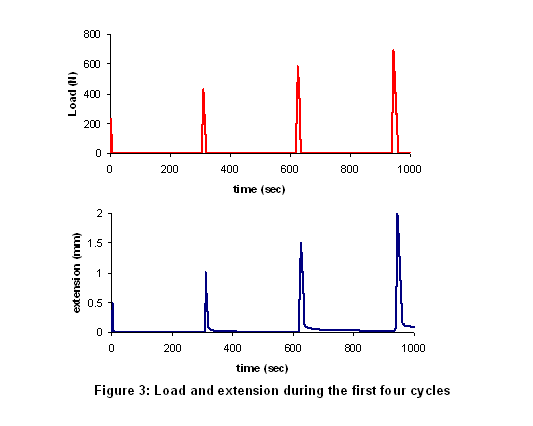 2nd cycle: Step1: the extension is brought to level Step2: The load is taken to zero and maintained at this value while the specimen is relaxing for 5 min. Cycles are repeated using increasing initial strains. Using a fresh test specimen, a stress-strain curve with extensometry was also generated in conformance with ASTM D638. Data Reduction From the stress-strain experiment, engineering stress-strain curves were calculated. Following Perkins (2005), the relationship between strain and cross-head displacement as plotted in Figure 4 was used as a means to correlate crosshead displacement to strain in the relaxation experiments. 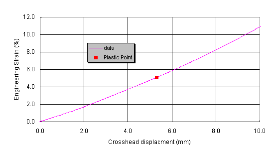 The relationship between engineering strain and crosshead displacement (extension) is observed to be fairly linear as can be seen in the plot and appears to hold well until the non-linear post yield region where necking behavior begins. The residual crosshead displacements after 5min of relaxation were converted to residual strain using Figure 4. The imposed crosshead displacements were similarly converted to imposed strain. The resulting data is shown on Figure 5. 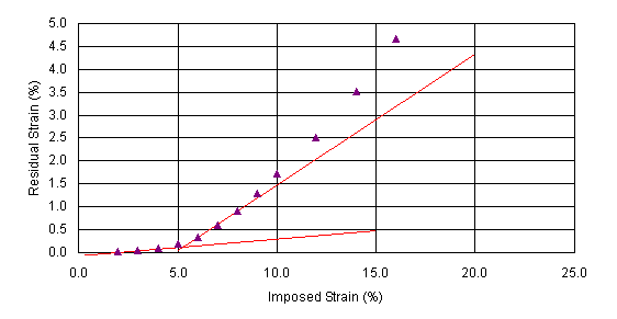 The residual strains at low imposed strains are low and linearly increasing. These residual deformations correspond to residual viscoelastic strains, meaning that they would tend to zero over time. For larger imposed extensions (around 4-5 mm), the residual deformations become significant, as some plastic residual strains are also accumulated. To measure the plastic point from the curve, the initial few points are fitted with a straight line. The plastic point is the imposed strain at which where the data deviates from the straight line by a fixed percentage. To increase the accuracy in the region of interest, additional data points can be obtained. The plastic point is plotted on the stress-strain curve in Figure 6. The polypropylene material shows a very dramatic transition from essentially elastic behavior to plastic behavior at about 5% strain whereas its yield point is at around 10%. This points clearly to the importance of knowing the plastic point and using it as a fundamental basis for placing stress limits on a design. The plastic point could potentially have implications related to endurance life and stress recovery. 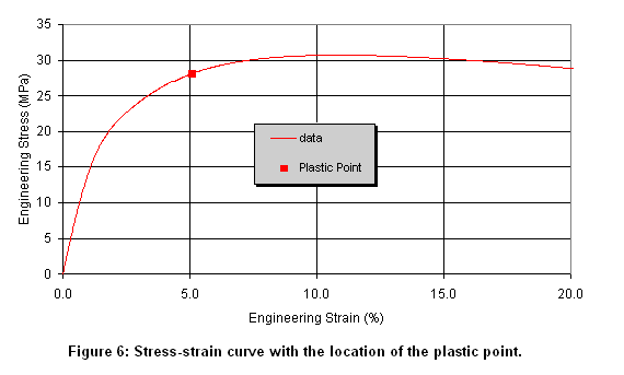 Material Modeling The experimental data presented in the previous sections clearly illustrates the complex behavior exhibited by plastic materials. This behavior cannot be represented accurately with classical plasticity constitutive models that are based on the assumption of small elastic strains and linear elasticity. In this section we address the complex behavior of plastic materials using a kinematic framework based on the multiplicative decomposition of the deformation gradient into elastic and plastic components: The isotropy assumption implies that the elastic strain energy potential can be expressed as a function of the principal logarithmic elastic strains (Simo, 1992). We adopt the following form of the elastic energy function: Here It is noted that the separable form of the proposed strain energy potential corresponds to an extension to nearly incompressible materials of the Valanis-Landel hypothesis (Valanis and Landel, 1967). It can also be viewed as a generalization of Ogden’s function, with the essential difference that no specific forms for the functions F and G are adopted here. Instead, these functions are determined directly from experimental data using a numerical procedure developed by Hurtado. Problems of finite strain elastoplasticity are more conveniently formulated in terms of the Kirchhoff stress measure. The Kirchhoff stress, r, is related to the Cauchy (or true) stress, The classical Mises yield condition takes the form: Here denotes the deviatoric part of a tensor, The basic procedures for the calibration of the material model are discussed next. Specifically we describe the methodology used to determine the hardening curve, In a uniaxial test, the following relationship exists between the Kirchhoff stress, the nominal stress, In a tensile test, 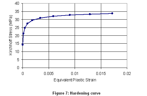 The elastic response of the material is characterized with the relationship between the applied Kirchhoff stress and the logarithmic elastic strain 
Figure 8 shows the curve of Kirchhoff stress versus elastic strain of this material for the uniaxial tensile test. This curve was used to compute numerically the functions F and G in the elastic strain energy potential in Equation 1. 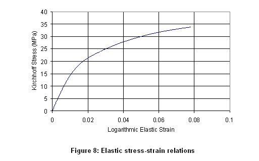
  Future Work In the next step, further validation of the model will be performed under more complex loading conditions. At this stage, the following validations are envisaged:
The authors wish to acknowledge the contributions of Francois Barthelat, formerly of DatapointLabs, for his involvement in the early stages of the work and in the design of the experimental schemes used for the tests. Thanks to Brian Lussier, DatapointLabs for performing the experiments and to Brian Croop, also of DatapointLabs for the data reduction calculations. We are also indebted to Kunming Mao, of ABAQUS Central, for numerous discussions on material modeling aspects. Last but not least, the comments and advice of Anita Bestelmeyer of Becton Dickinson and Don Jagos of Visteon were invaluable in setting the direction of this research. References 1. Courtney T. H. “Mechanical Behavior of Materials”, McGraw-Hill Series in Material Science and Engineering (1990). 2. Perkins L.R., Lobo H., " A Novel Technique to Measure Tensile Properties of Plastics at High Strain Rates" SPE ANTEC Proceedings, Boston (2005) 3. Quinson R., Perez J., “Components of non-elastic deformation in amorphous glassy polymers”, Journal of Material Science 31 p. 4387-4394 (1996) 4. Quinson R., Perez J., “Yield criteria for amorphous glassy polymers”, Journal of Material Science 32 p. 1371-1379 (1997) 5. Simo J.C, “A framework for finite strain elastoplasticity based on maximum plastic dissipation and the multiplicative decomposition: Part I. Continuum formulation”, Computer Methods in Applied Mechanics and Engineering 66 p. 199-219 (1988 a) 6. Simo J.C, “A framework for finite strain elastoplasticity based on maximum plastic dissipation and the multiplicative decomposition: Part II. Computational Aspects”, Computer Methods in Applied Mechanics and Engineering 68 p. 1-31 (1988 b) 7. Simo J.C, “Algorithms for static and dynamic multiplicative plasticity that preserve the classical return mapping schemes of the infinitesimal theory”, Computer Methods in Applied Mechanics and Engineering 99 p. 61-112 (1992) 8. Simo J.C, Hughes T.J.R, "Computational Inelasticity", Springer-Verlag, New York, 1997. 9. Valanis K.F. and Landel R.F., “The strain energy function of a hyperelastic material in terms of the extension ratios”, Journal of Applied Physics 38 p. 2297-3002 (1967) |
|